EpiDiP User Manual
Table of Contents
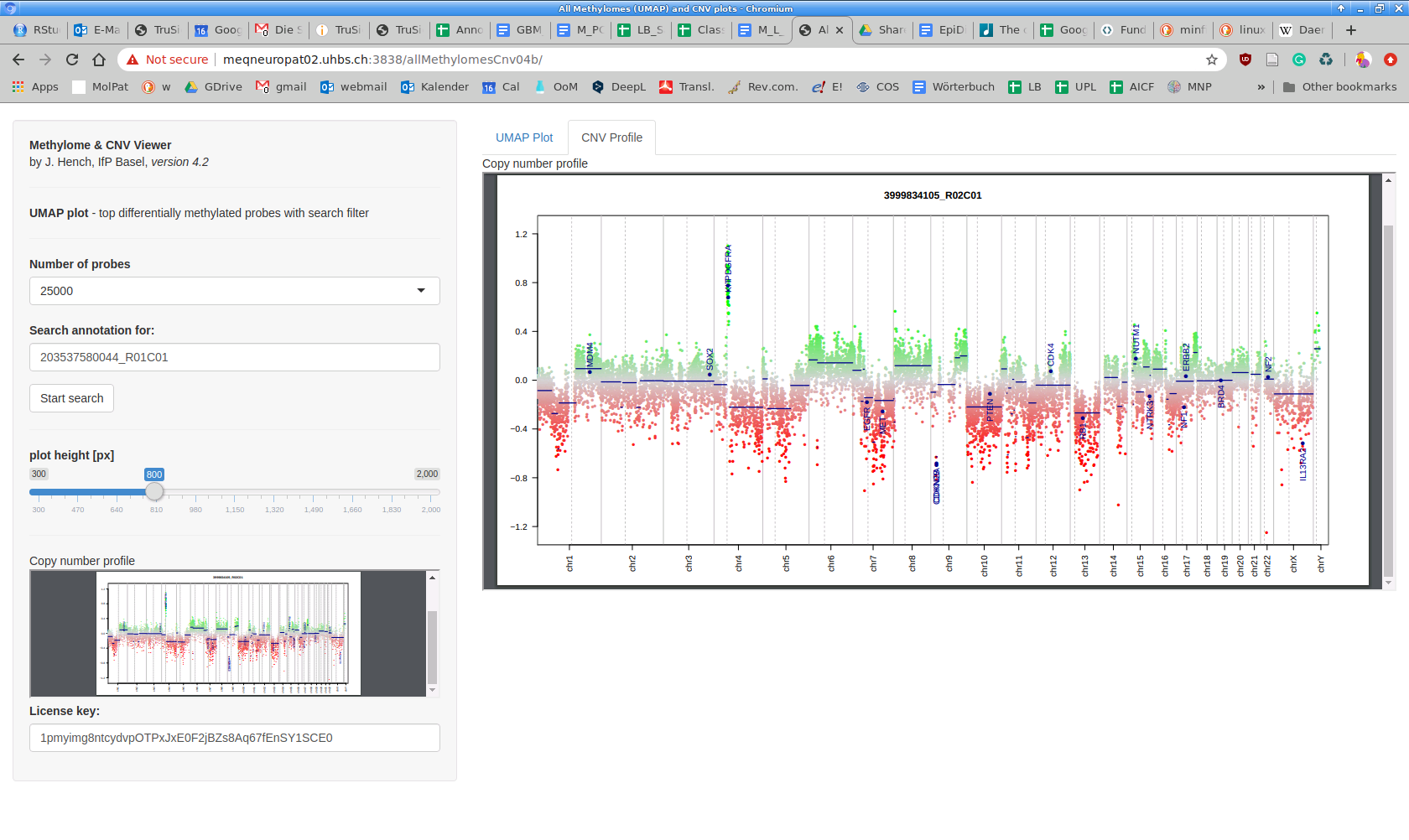
Interactive Methylome & CNV Viewer
Since 2017, we have been employing the Heidelberg Brain Tumor Methylation Classifier (www.molecularneuropathology.org) in routine tumor diagnostics at the Institute for Medical Genetics and Pathology, University Hospital Basel and University Basel, Basel Switzerland. As described in the original paper [1] dimension reduction by tSNE can be particularly helpful when established classifiers fail to render a reasonable diagnosis. Mostly such unclassifiable cases comprise metastases from extracerebral neoplasia, low tumor cell content biopsies as well as biopsies with degraded DNA, and, importantly, entities not yet trained in a classifier. To overcome these limits, we processed large portions of publicly available methylation data from TCGA and GEO that we currently consider suitable to support our EpiDiP (Epigenomic Digital Pathology) tool.
The data lake we maintain has been normalized and converted into a 450K array-like format (through minfi / SWAN) with approximately 400K probes. For each methylome dataset, a chromosomal copy number profile is plotted and annotated with selected genes for a quick overview (through conumee). Currently, only 450K and EPIC arrays (Illumina Infinium Methylation) are considered. For dimension reduction, we find UMAP more efficient than tSNE. The frontend, also created in R, relies on Shiny and Plotly. By offering (and maintaining) this platform free of charge, we hope that colleagues around the globe will find our tool useful in helping their patients.
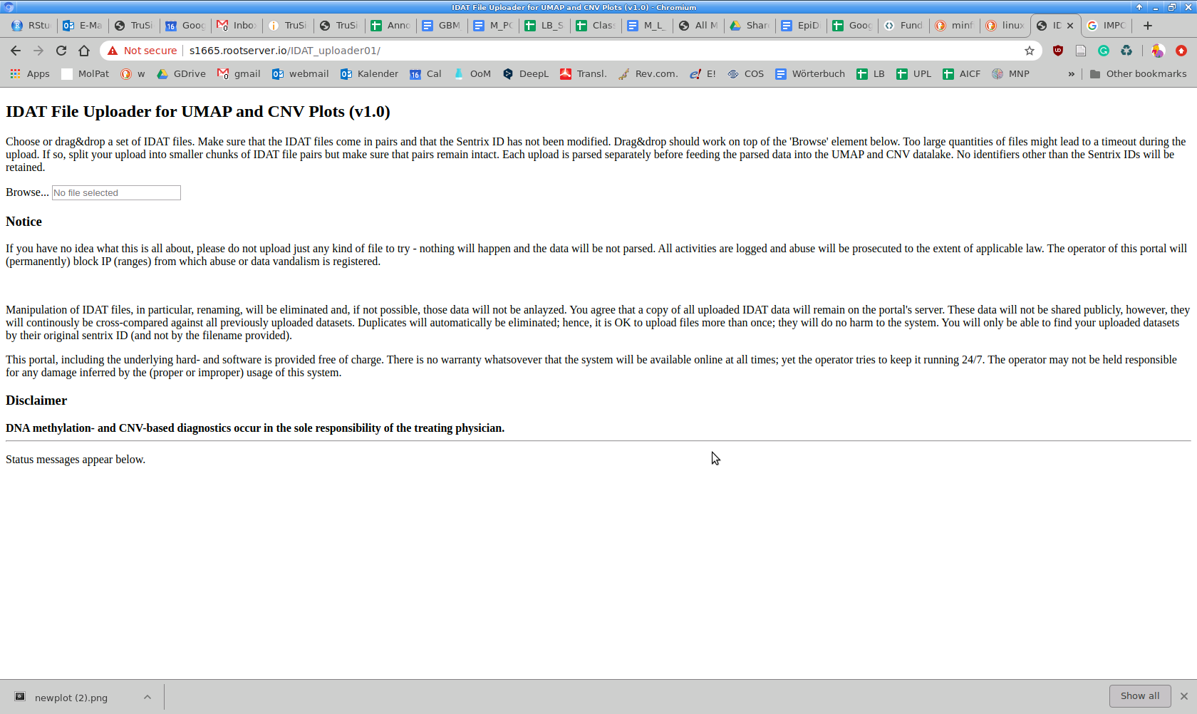
EpiDiP is provided "as is" and free of charge but comes without any warranty. It is not clinically validated. DNA methylation- and CNV-based diagnostics occur in the sole responsibility of the treating physician.
The Methylome & CNV Viewer comes in two versions that are located on two different platforms. One uses http (port 80), the other https (port 443). Both are functionally equivalent but might respond differently when site blockers are in place (e.g., inside hospitals, for security reasons). Hence, if one of the two works for you, there is no need to use the other platform. Our tool has been tested with several web browsers: it seems that chromium/chrome work best, in particular, due to their integrated PDF viewer. Firefox also comes with a PDF viewer, but since copy number plots are vector graphics with many elements (one per probe), rendering is very slow compared to chromium/chrome. If you experience any prolonged lags, this is typically due to your browser, low RAM on your local machine, or both. If the viewer does not load at all, firewalls and other blockers might be in place. Try alternating the http/https versions to alleviate the problem.
The key operation elements have a "pop-up help", i.e. when hovering the mouse over one of these elements, a short description will appear.
Before running UMAP on the data lake, a choice of top differentially methylated probes is autonomously made by the software. To directly compare 450K and 850K array data, an overlap probe set of approximately 400K probes is created. Cross-reactive probes, as determined for the 450K array [2], are removed; sex chromosomes are ignored [1]. Resulting data are annotated in 450K probe nomenclature through the minfi conversion function. Currently, you can choose between 25K, 50K, or 75K top differentially methylated probes (based on a standard deviation-based ranking, [1]). Once you have made a selection, the UMAP plot reloads. It is not possible to maintain the current zoom level during reloading.
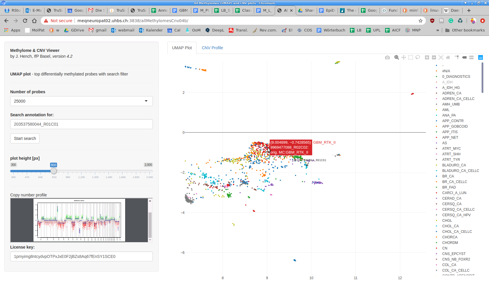
Annotations are represented as lines in the "Sample List" table of the submitted Google sheet. The search tool is, in particular, intended to search for individual (e.g., diagnostic) cases by their unique Sentrix ID. Internal sample names (e.g., a biopsy number in a custom annotation) or text within the "Classifier diagnosis" field can be searched as well. Note that this is a case-sensitive plain text search acting on a concatenated string of the respective annotation (no wildcards). Identified case(s) will be highlighted in the plot by a static arrow mark.
The feature can also be used if keywords were added to the annotation that occur only in a subset of cases. However, in most instances, it may be more straightforward to define an additional methylation class in a custom annotation specifically for this purpose, which leads to a uniform coloring of all cases belonging to this new methylation class.
The "Search annotation for" box requires the "Start search" button to be clicked once. Execution can take a moment since the server reloads the Google sheet for each search.
This field contains the Google sheet ID for the currently loaded annotation. You can use our public annotation which contains all of TCGA's and many of GEO's freely available data sets. We modified this annotation to become particularly useful for Cancer of Unknown Primary (CUP) diagnostics. Please note that our annotation is far from perfect, and we continue to identify wrong, misleading, or outdated annotations (e.g., you will still encounter many LGG OAII (lower grade glioma, oligoastrocytoma WHO grade II) and find some of them in the oligodendroglioma (IDH mutant), astrocytoma (IDH mutant), or glioblastoma (IDH wildtype) clusters. If you wish to improve the annotation for these cases, please let us know. For the time being, especially in the above-mentioned scenario, it is often helpful to consult copy number profiles by clicking on a case dot. To create and curate your own annotation, please consult the respective section.
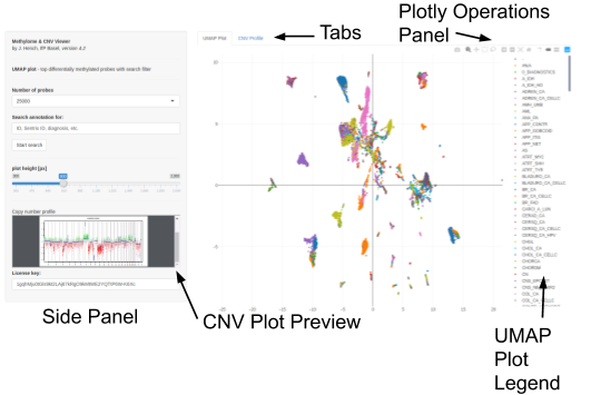
When loading the Methylome & CNV Viewer, the preview area will become visible once a dot in the UMAP plot is clicked. This will invoke the PDF viewer within your web browser. By default, it will show the plot as a thumbnail preview. If instead, your system PDF viewer shows the plot, you might need to change the defaults for PDF documents to use the integrated viewer in your web browser's preferences and then reload our web application. The browsers currently working best are chromium/chrome. The "CNV Viewer" tab shows the same PDF but allows a more detailed view. While it is generally possible to create PDFs with any locus annotated in conumee, this is currently not possible through our online tool. The creation of a dynamic CNV Plot Viewer with locus search functionality is in progress. As computing CNV plots is computationally intense, we have precalculated all plots. All incoming files will be plotted only once upon entering the data lake. Please consult the conumee vignette to find out how to generate your own CNV plots.
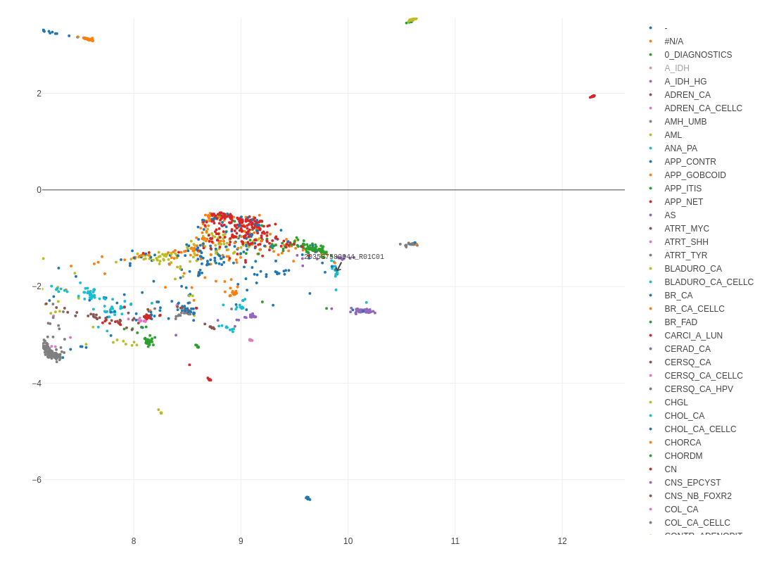
UMAP plots are displayed through Plotly. The Plotly package generates a legend on the right side and a graphic menu with zooming and panning functions on the top right corner of the plot. Performing a double-click on a single entry in the legend will hide all dots except for those belonging to the double-clicked annotation. Single-clicking one of the hidden (greyed-out) entries will additionally show all dots belonging to these entries. It can take a moment after each click / double click until you will see a change. Note that operations inside the Plotly-based UMAP plot are overridden by the functions in the Side Panel that almost always reload the plot. After reloading the plot, all settings, selections, annotations, etc. inside Plotly are reset to defaults.
Hovering the mouse over a dot (representing a particular methylation profile) shows the Sentrix ID, the Methylation Class, and the Classifier Diagnosis fields from the currently loaded annotation. For non-annotated cases (Methylation Class = "-") only the Sentrix ID is displayed. Since >15'000 dots are plotted with their annotations (only visible upon hovering), it always takes a moment for the UMAP plot to refresh. It also consumes quite a bit of web browser memory (dependent on browser/OS combination); in case of hangups/timeouts, please reload the web application in your browser.
Clicking on a single dot (e.g., after zooming in using Plotly's menu on the top right side) loads the corresponding CNV plot. Depending on server load, it can take a few seconds for the CNV plot to load, in particular in the https version (here, the PDF is requested from our server to be sent to the public shinyapps.io server which, in turn, serves it to your browser).
You can also create screenshots through Plotly's menu; however, their resolution is quite limited. As an alternative, taking screenshots with an external application on your computer might produce prettier results.
Due to restricted computation time on our "outposts" (i.e. rented web server, limited shinyapps.io webspace) it is currently not possible to locally save an interactive UMAP plot from our system. Furthermore, interactive Plotly plots embedded in HTML files do not support linking to CNV plots as in our web application.
This tab contains a larger version of the embedded PDF viewer. Switching back and forth from the UMAP Plot tab does not change the current view. All functionality provided in the Side Panel remains active and acts on the UMAP Plot tab. If CNV plots are not displayed correctly as shown, this is most likely due to your current PDF handling configuration. "Not found" errors in the PDF viewing areas are likely due to an update of the UMAP plot which occurs about every four hours. In such cases, please reload the web application.
The IDAT Uploader is a Shiny application that supports file selection from the local computer by either the "file open dialog" referenced by the web browser and operating system or, alternatively, allows to drag & drop multiple files (not folders) onto the "Browse" button.
This button may look a bit different depending on the browser/OS combination. For instance, when using the Chromium browser on Linux, the button does not even appear as a "button" but you may still click on "Browse…".
Since the system works without password protection or alike, we had to put some security measures in place. Most prominently, these subroutines only consider files with an expected file size as valid and require that they are uploaded in matching pairs (within the same upload). Hence, uploading "red" and "grn" IDAT files separately will cause these files to be ignored. For the ease of use (we hate if we have to click more than necessary), it is possible to dump an entire array folder that contains multiple pairs of IDAT and potentially other Illumina files we don't need to process. They will all be uploaded (consuming a bit of bandwidth), but only matching IDAT file pairs will be considered for analysis. The “file open” dialogue can be useful in such situations as it filters for the ".idat" suffix. Multiple files can typically be selected with SHIFT-click or CTRL-click. Upon upload, a progress note will appear below the "Browse…" button. After the upload has been completed, a status message will appear at the bottom of the website. You can now upload further files or close the browser tab.
It is currently not possible to display the progress of analysis. The UMAP daemon process is continuously running in an infinite loop. It takes about 3 hours (depending on all unrelated computational loads of our computer) to calculate the UMAP plot for all files in the data lake.
UMAP is an unsupervised machine learning algorithm. As such, it does not consider any annotations; it compares subsets of raw data against each other. These subsets are defined through several filters (see Interactive UMAP & CNV Viewer). The coloring of case dots in the UMAP plot comes from an annotation, which is read during re-plotting. To ensure a highly flexible data input, we decided to use the Google Sheets platform. While it might not be obvious at first glance why Google Sheets are more straightforward than managing data in a local database or even flat files, data management using this highly tracked system is beneficial for all for several reasons: the Google drive platform behaves (at the user side) like a giant database server. Every "document" (note the "") created on Google drive gets a Google-internal ID, which is unique worldwide (!). Also, Google "documents" are versioned, i.e. every change to them is recorded, with a version history for each document that includes when and who modified what. Therefore, we consider Google sheets practical for maintaining a managed, up-to-date working copy. Documents can be created on a per-user level and shared with others at different access levels (read-only, comment = track changes, edit) through their IDs. Google document contents can also be downloaded (through https) in several file formats including Microsoft Excel (XLSX). Download links look like this:
https://docs.google.com/spreadsheets/d/1gqhMju0tGls9kt2LAj67kRgO9kMtWE2YQTtP6W-K6Xc/export?format=xlsx
The marked red passage is the document ID, as it also appears in your web browser's address/URL field. Our Interactive UMAP & CNV Viewer takes the Google document ID from the field License key and tries to temporarily download the referenced document in XLSX format. If it does not succeed, the application gets an internal error and is terminated. Since Shiny immediately processes user input (without pressing "enter" or alike), a key can't be written into the field but must be pasted over the existing one: select the document ID of your Google sheet in your web browser’s URL field, copy it to the system clipboard (CTRL+C / Apple+C), place your cursor in the License key field, and execute "select all" (CTRL+A / Apple+A). Then paste the new key into this field (CTRL+V / Apple+V), and the plot should start reloading with your new annotation. Your annotation is only transferred to temporary memory on our server but not stored there. It is reloaded from your shared Google sheet every time the plot reloads. If you wish to share your annotation with us, you can do so by sending us the URL to your shared Google sheet via email.
It is also possible to "live merge" Google sheets within the Google sheets editor. We use this feature to create merged annotations that are based on different sources. The key function is IMPORTRANGE. Please consult the Google sheets help on how to use it. In short, this function can link a range of a sheet through its URL (i.e., sheet ID) into another. You could, e.g., import the relevant columns from our sheet into a sheet in which you also maintain your own diagnostic annotation. We are currently working on a template Google sheet document to automate this process even further.
We curate a list of methylation classes in our google sheet and share a list of annotations. This table explains the methylation class short codes in the Interactive Methylome & CNV Viewer. Sometimes, the annotation source is listed with particular cases, and in some instances, mismatches of annotations are present. Usage of the Basel annotations occurs at your own risk.
[1] D. Capper et al., ‘DNA methylation-based classification of central nervous system tumours’, Nature, vol. 555, no. 7697, pp. 469–474, Mar. 2018, doi: 10.1038/nature26000.
[2] Y. Chen et al., ‘Discovery of cross-reactive probes and polymorphic CpGs in the Illumina Infinium HumanMethylation450 microarray’, Epigenetics, vol. 8, no. 2, pp. 203–209, Feb. 2013, doi: 10.4161/epi.23470.
The EpiDiP backend is largely written in R and runs on a multithreaded multicore Linux computer (x86_64, 120 threads, 2TB, currently). A GPU port using gpumap, written in Python, has been released 2020-07-30 and runs on an NVIDIA RTX 2070 with 8 GB RAM.
BTW: Our logo represents the nature of epigenomics, acting like DIP switches on top of DNA (instead of historic computer board BIOSes). This entirely unrelated terminology fits our computational strategy in "Epigenomic Digital Pathology" - EpiDiP.
last updated 2020-07-30 by Stephan Frank & Jürgen Hench
.jpg&sa=D&ust=1596107480625000&usg=AOvVaw33i79m_9kFQ9m3EZV0DSib)